Recently AlphaFold2 released a new batch of models, this time covering all of the Trembl sequences in Uniprot, resulting in a huge number, which got hashtag-academic-twitter and some news editors very excited for the stamp-collecting feat. Personally, I find it annoying, not because it's pointless, but as of writing this, it has made any search for a target by name swamped by irrelevant sequences.
However, AlphaFold is great for other feats.
I have blogged about it a few times (e.g. link), which gives away my positive view of it! It can predict oligomers, with a lot more precision and confidence than docking. It does not always work either technically or meet the hypothesis. I did a long series of experiments with a hypothesis in mind which wasn't valid in the end (here), but revealed novel science and took a few minutes to set up and a few hours to run, which would have taken years if done by Western blot of a co-immunoprecipitation or cross-linking mass-spec.

First a disclaimer: I have never run a Western and the last time I held a pipette I had to be reminded how to hold it (release button rests towards one's thenar webspace), so I am not sure years is accurate.

ColabFold

A corgi wandering on the top of a colab notebook
(Atlas for comparison)

ColabFold is a descendant of sorts of AlphaFold's colaboratory notebook, which has a faster MSA step, easier sequence input syntax and more accessible devs. It is meant to be run on a Google Colaboratory notebook, but it totally can be run in a Jupyter notebook or in bash.

Showcasing ≠ everyday use

Google Colab is a great way to showcase tools, but not necessary use. For Fragmenstein I have made a Colab notebook as a demo for the manuscript and shared it on Twitter. This is a very powerful tool as it's a form of "try before you buy" and is well received (if a picture thumbnail is provided for the initial attention grab). I do not use Colab for ColabFold, but a remote Jupyter-lab notebook, but the tool is the same (with some minor changes), which I discuss in a separate blog post TBC. The benefit is power and tidiness, but the disadvantage that Jupyter notebook does not allow wandering corgwn on the title bar, but has the advantage one can use much more compute power.

Spaghetti

With a model from EBI-AlphaFold2 there are a few things to look out for as discussed here. Briefly, the off-the-shelf model is a monomer, which may not be biologically real, and it may have long low confidence loops dubbed "spaghetti", which may bind "something" (see below). This is exceptionally common in transcription factors, which recruit the mediator complex and can bind it in one of a dozen sections given it is such a big protein.
A key concept to discuss is the confidence metric. The model quality is measured in pLDDT, which is available per structure, per residue and between residues. The latter goes into making the green plots in the AF-DB, while the middle replaces the b-factor column and below 70% has low confidence. Parenthetically, the quality metric pLDDT is written with a lowercase L for local in its original paper, but l is ambiguous with I, so most places seem to rightfully not adopt the original use. It's rather like in Klingon (thıngan Hol), where all i are uppercase, which confuses people hence why they angrily glare when seeing a message in Klingon on social media —those petaQpu'.

Colour hexes

Parenthetically, one may want to copy the colours used by EBI-Alphafold2, which are not CSS primary colours as some snippets online claim. These are:

The blue colour is #0053D6 (pLDDT ≥ 90)
The cyan/teal colour is #65CBF3 (90>pLDDT≥70)
The yellow colour is #FFDB13 (70>pLDDT≥50)
The orange colour is #FF7D45, pLDDT<50)

(It is not a gradient nor is it a linear shift in hue —it would go blue>teal>green>yellow>red if it were).
To apply this in PyMOL, the command is:

color 0x0053D6, element C
color 0x65CBF3,  b < 90 and element C
color 0xFFDB13,  b < 70 and element C
color 0xFF7D45, b < 50 and element C

To make loops more sausage-like the command set cartoon_loop_radius, 1 will do the trick.

However, there is more to pLDDT than pretty pictures. In fact, protein-protein complexes may involve these spaghetti loops and if they do, the span involved may likely have a confidence in the 70–40 range, while the rest of the spaghetti loop is less than 40. As we will see.

The unexplored complexes

Having gone over pLDDT, let's talk about complexes.

I often get asked what does a given residue do. I streamlined this task into Venus, but all too often I end up with a surface residue, where I have to hunt down the binding partner. I will admit that I do not do all the reading I am meant to do, but instead read the blurb in the Uniprot entry, read an abstract or two, search for figures of that protein and look on PDB for what models in complex are available.

Parenthetically, the latter step can be a slow unless optimised, but in my opinion one should not overdo it as one loses oversight. It can be automated with the packages pypdb, requests (for the simple PDBe API), bio.pairwise2 and pymol2 in Python, but is beyond the scope of this post and is tricky anyway (species, ranges etc.), so doing it semi-manually is actually more convinient. What I do is go to RCSB PDB in a browser, search for protein name, click on the tabular report dropdown, chose custom and add only Macromolecule Name (or with Molecular Weight (Entity) if I don't want peptides. This gives a table of PDB entry and the protein they contain. If needed Uniprot data can come from SIFTS which is easy to query automatedly. The chosen parts can be assembled into a PSE with the Python package pymol2, which then can be opened for viewing with PyMOL binary. Even when including paralogues and checking SWISSMODEL (and stealing partners from the templates) one however often only gets only a limited number of interacting partners. Luckily, AlphaFold2 and friends save the day. A nice example of a complex series of interactions is the ubiquitination pathway in Eukaryotes discussed below.

Before AlphaFold2, the main tool was protein-protein docking —cue initial brass fanfare from Richard Strauss's Also Sprach Zarathustra.

Docking consists of finding the conformation of complex with the lowest potential energy. A series of decreasingly weaker poses are returned and generally looking at the top ten should give consistent picture and a very low ∆G_bound. The former is rarely true and the latter is a very hard to contextualise number —remembering that one hydrogen bond is 1 kcal/mol and a salt bridge is 2 kcal/mol helps, but it does not really as larger protein give larger values.

The problem is that protein are somewhat flexible and many interactions are water mediated. The classic example is barnase+barnstar: the interaction is really strong (–19 kcal/mol), but involves lots of water mediated hydrogen bonding. Googling images for this pair will reveal endless graphs showing how complicated this is to predict. ColabFold on the other hand is different. I hate to say it, but it does not molecular thermodynamics and instead revolves around residue covariance and a well trained model. Consequently, it will spot the residues that show epistasis, but will not give a damn if they form water mediated bonding or not —actually, without the final AMBER step one often gets overlapping sidechains at the interface. With ColabFold a dimer will either resolve consistently across models or will be floating in random locations, with rarely cases in between.

In another post and in the associated notebook, I talk about calculating the Gibbs free energy of the interface. Molecular thermodynamics calculations definitely come in handy to test certain hypothesis. For example, in a model I made of a certain protein the interaction was 5/5 consistent except for a bit of change in angle for two out of five due to an everted loop. When the models were phosphorylated with PyRosetta using data from PhosphoSitePlus, it yielded a stronger interface for the everted loop. This is interestingly scAfter all showing alternate conformations is a main strength of AlphaFold2.

Ubiquitination, an example

The ubiquitination system is a great example of the power and limits of AlphaFold2. In the canonical ubiquitin-conjugation system, the C-terminus of ubiquitin is ligated to the sidechain of a lysine via a first enzyme E1 in an ATP dependent manner, which is then transamidated to a carrier E2, which passes it to E3 which passes to the target protein, which is generally presented thanks to an adaptor protein. ColabFold will make a great E1+ubiquitin, E2+ubiquitin, E2+E3+ubiquitin and E3+ubiquitin models, wherein generating 5 models will result in very consistent binding positions (>3 Å RMSD). A problem arises with substrates and adaptors: the diverging paralogues bind different targets, which will not be linked together correctly in the MSA, resulting in loss of their covariance signal.

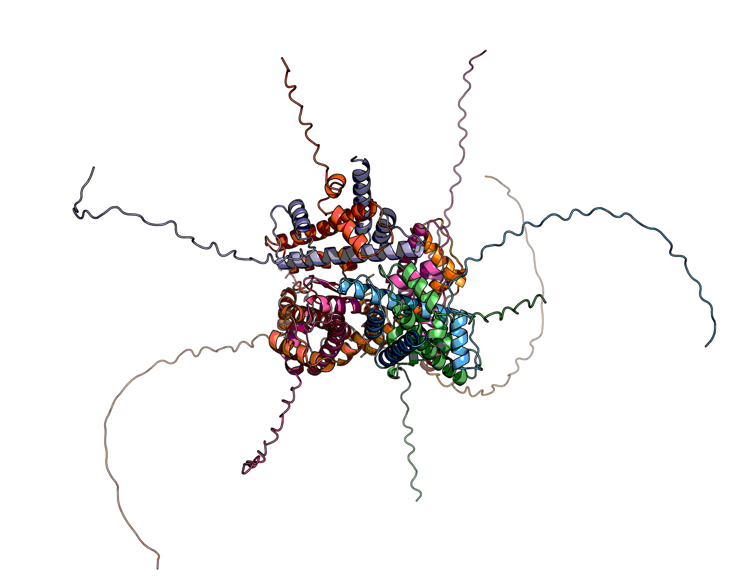
Recently, I was asked whether a given residue is an interface residue with a given binding partner. Autophagy is controlled by a series of protein (with names in the form ATG👾, where 👾 is a number), which act like the ubiquitination system, with ATG12 as the ubiquitin tag, but actually an adaptor. ATG7 is the E1 ligase (ATG dependant first step), ATG10 is the carrier to which the tag is passed, ATG5 is the E2 ligase, which accepts the tag. But does not pass it to a final substrate binding E3 ligase, but instead binds to a localisation scaffold (ATG16) and a target (ATG8 via ATG3) into order to bring it into place for myristoylation thus altering membrane curvature. This process is inhibited/interfered-with by ASPP members, which have an internal ubiquitin-like domain, which is know to compete with ATG12 for binding to ATG5. So I started off looking at diagrams and testing a few things, which led me this model:

In a first model I was not expecting ATG10 to bind where ATG16 binds, but that makes sense and is possible thanks to the long C-terminal domain of ATG12 (and ubiquitin). Curiously, this means that ATG7 can still bind when ASPP is bound as it is on the opposite side.

This all sounds great. However, things do not often go as hoped. A common case is that the protein are not sticking together or if they are they are not sticking consistently.

Troubleshooting

I do not know what works best for a given situation, but there are three routes:

Tinker with the sequence
Tinker with the settings
Tinker with the MSA

In fact, I made a joke bingo card to check off for things tested. Most of the cells are jokes. Whereas the onomori from the Kanda shrine in Akihabara, Tōkyō, are phenomental, I would not considering going to the effort of sourcing them in Europe a good strategy...

Reinstalling the environment is a good tactic if there's an actual error, but generally with everything tensorflow related, a seemingly innocuous package installation can inexplicably result in the waste of a good chuck of time firefighting, so a reinstall is not too wise.

Sequence: remove spaghetti

The longer a sequence is the more places things can go wrong, so removing end domains that do not matter or removing spaghetti loops can help. For example, here is a complex (unrelated to ubiquitination), where the accuracy goes up by trimming the tail spaghetti (5 models):

If the spaghetti loop is in the middle of the protein, then there are four options:

Split the protein in two separate peptides
Replacing a long span of residues with a series of glycines (gap distance divided by 3.4 Å with an extra 20–50% should suffice)
Edit the MSA as an A3M has insertions simplified —very complicated
Use an older colabfold notebook, wherein cuts within a protein were maked with a / —this is a bad idea

As mentioned earlier not all spaghetti is junk. Some may be involved in protein-protein interactions. These represent a very small fraction of the PDB so AF2 performs badly at predicting these, but can still managed in some cases —followed by cycles of refinement. AF2, however, can possibly improve on PDB models. For example here is a certain protein bound to tubulin alpha and tubulin beta as predicted by ColabFold: in the PDB model, a dodecapeptide is bound, while in the models a 24-mer (icositettarapeptide) is bound but actually 2 of 5 are different residues (binding in the same way) as it's a repeat so in reality would bind 4 tubulin monomers.

Linguine

In isolation the binding sequence is a disordered spaghetti loop, but as mentioned there seems to be a difference in confidence in these regions, and in fact other disordered regions with higher than 40 pLDDT bind other targets, I call these linguine loop:

Interdomain loops

A curious case is interdomain loops. If the pLDDT is very low on the segment removed then there is little change of harm. The only consideration is that the remaining parts ought to be able to close up —measuring the distance in PyMOL between the good residues (edit mode>click on the two atoms or type print cmd.distance('name CA and resi 👾', 'name CA and resi 👾) and dividing it by 3.6 and multiplying that by 1.5, should give a rough number of residues required.

Another caveat is that if the alignment is generated by blasting and only the first HSP is taken per hit, even if the HSP are non-overlapping, there will be a bit of the alignable hit missing. MMSeqs2 does not use Blast, but HMM (cf. HH-suite) on a pregenerated dataset of clusters so this does not apply.

The major catch with removing termini or removing inner loops is that it becomes complicated to keep track of the sequence, when one want to convert the model back to the correct numbering.

To correct the numbering in PyMOL, say in chain B by 100 residues, one can do alter chain B, resv+=100, followed by sort. If one has forgetten what the protein splicing was, the a global alignment can do the trick, as happens in this function: link.

Splicing

A detail to note about interdomain loops is that these may be because a non-biologically relevant splicing isoform is chosen.

When a non-biologically relevant isoform is used, the differing sequence will be a disordered spaghetti.

Unirpot is nice for choosing the isoform which is most frequently found in transcriptomics experiments, while Ensembl choses the longest, which may not be relevant.
The database GTex is a really nice resource for doublechecking this is correct by showing the abundance of mRNA reads spanning junctions and the exons are found in human tissues —as the genes can be big and the reads small it does require some squinting at times. To play around with the sequences of all the possible isoforms in Python the local ensembl package can help, for example, here is their sizes:


# remember local data...
!pyensembl install --release 77 --species homo_sapiens

from Bio import SeqUtils
from pyensembl import EnsemblRelease
data = EnsemblRelease(77)
ts = data.transcript_ids_of_gene_name('ALG13')
transcripts = [t for t in map(data.transcript_by_id, ts) if t is not None and t.protein_sequence is not None and 'X']
for t in sorted(transcripts, key=lambda t: SeqUtils.molecular_weight(t.protein_sequence.replace('X', 'A'), 'protein')):
    print(t.transcript_id, len(t.protein_sequence), SeqUtils.molecular_weight(t.protein_sequence.replace('X', 'A'), 'protein')//1_000)

A side-effect of this is that one would want the other sequences in the MSA to be correct or else the quality will be poor.

Sequence: try different domains separately

In generally, longer protein will require greater resources. Therefore, splitting a protein into domain is a very solid plan. In terms of complexes, this may help, although it will result in different MSAs, which can be counterproductive for repeat proteins.

Settings

One can also increase the number of recycles, which is how many cycles are done, which is generally considered a good choice. The AlphaFold2 paper performs 3 recycles, but one can do a lot more. These simply increase the time requirement (linearly I would guess).

There is also the option to use templates in ColabFold. These are for specific applications (e.g. alternative conformations or novel structures), not for giving ColabFold a hand. ColabFold has to rediscover structures it already predicted, there is no circumventing that: it actually runs slower with templates. And I suspect it uses in a fragment based approach, because when I altered all non-glycine/proline residues to alanine in a ubiquitin structure (PDB:1UBQ, file of the heretical structure) and used its sequence as sole alignment I got the same helical structure repeated:

Personally, I have not had much luck with templates, but I am told they could help.

MSA

The MSA is a key part and can play a massive role. In a GitHub I have put a few snippets for working with A3M files, which can help. Here are some key take home ideas.

A3M

Cardinality of a protein
does not involve RC clergy

An A3M alignment looks like a normal Fasta formatted alignment, but with two differences.

For a complexes, the first line starts with a hash and is immediately followed by the comma separated lengths of the peptides, then a tab, then the comma separated cardinality (oligomeric number) of the peptides.
Insertions in the non-target sequence are marked with lowercase letters and the target sequence does not have gaps for them.

To convert a regular Fasta alignment to a A3M one, in the HH-suite repo there is a Perl script for this:

wget https://github.com/soedinglab/hh-suite/raw/master/scripts/reformat.pl
perl reformat.pl fas a3m out_al.fasta out.a3m

Uniprot

One detail that should be noted is that in a ColabFold-MMSeqs2 MSA the sequences are Uniprot and/or environmental. Uniprot is really good for curated human protein as these are curated and user-submission curated —I have messaged about a few mistakes I have spotted and within a week I got a human thank-you reply and the page was altered. For other organisms this is less so, to the point that I have found NCBI much better in terms of gene length and presence. This is because a genome sequencing project for a non-human organism is rushed through the doors and is not subsequently re-refined as far as I understand. A case example is the lamprey, which featured heavily in my post about anthropocentric MSAs. Briefly, this fish is basal to boney fish and tetrapods and it's divergence predates two (tetrapods) or more (ray-finned fish like zerbafish) genome duplications. This ugly chap is useful because it has less paralogues, but is very poorly annotated in Uniprot.

A problem is that the Uniprot accessions are not too helpful for a human reader. Here is how one can get images of what is what thanks to Wikipedia using the snippets in the metioned GitHub:

from IPython.display import display
from gist_import import GistImporter
import operator
import functools
import pandas as pd
import ipyplot

# get codeblocks
gi = GistImporter.from_github('https://github.com/matteoferla/Snippets-for-ColabFold/blob/main/analyse_a3m.py')
AnalyseA3M = gi['AnalyseA3M']
gi = GistImporter('313b5c7e1845f36205b4b9dcf05be10d')
WikiSpeciesPhoto = gi['WikiSpeciesPhoto']

a3m = AnalyseA3M('👾👾👾👾.a3m')
a3m.load_uniprot_data()
df: pd.DataFrame = a3m.to_df()
wikis:pd.Series = df.species.apply(functools.partial(WikiSpeciesPhoto, catch_error=True, retrieve_image=False))
urls:pd.Series = wikis.apply(operator.attrgetter('image_url'))
pretties = wikis.apply(operator.attrgetter('preferred_name'))
ipyplot.plot_images(urls.loc[~urls.isna()].values, 
                    pretties.loc[~urls.isna()].values,
                    img_width=150)

Paralogues

The loss of signal from diverging paralogues ought to be correctable, but would require a lot of time to set up and I have not found an example of this being achieved or set it up myself. The MSA goes quite far back, allowing the conserved core of the protein to be resolved, but one can make a more shallower one. In another post, I discuss eukaryotic species choice and mention that for non-model organisms the number of missing genes or genes with shorter transcripts is rather high: for this MSA this does not matter, whereas genetic diversity does —i.e. mouse vs. human does little, whereas a series of fish become very helpful unless the double genome duplication gets in the way.
One rather crude way to remove paralogues is to filter out in the MSA all genes with the name that does not match a given criterion. From the GitHub repo of snippets:

from IPython.display import display

from gist_import import GistImporter
gi = GistImporter.from_github('https://github.com/matteoferla/Snippets-for-ColabFold/blob/main/analyse_a3m.py')
AnalyseA3M = gi['AnalyseA3M']

a3m = AnalyseA3M('👾👾👾👾.a3m')
a3m.load_uniprot_data()
omnia = a3m.to_df()
boney = a3m.to_boney_subset()
print(f'{len(boney)} out of {len(omnia)} are tetrapods & boney-fish')
a3m.display_name_tallies(a3m.to_boney_subset())
display(boney.sample(5))
# And do whatever filtering:
# names are messy...
cleaned = boney.name_B.str.lower()\
                      .str.replace(r'( ?\d+)$','')\
                      .str.replace(r' proteinous','')\
                      .str.replace(r' protein','')\
                      .str.replace(r'📛📛','📛📛2')\
                      .str.strip()
subsetted: pd.DataFrame = boney.loc[filtro & (boney.name_C == 'BH3 interacting domain death agonist')]
a3m.dump_a3m(subsetted, '👾👾👾👾_filtered.a3m')

Doing this on a ColabFold-MMSeqs2 A3M file will result in very few entries, which will not work. As a result one may have to resort to making one's own MSA.

Custom MSA

Honestly, I have not looked into creating a custom database for MMSeqs2 or its predecessor HH-suite, but I had used the classical method of simply doing a blast or psiblast search in NCBI and making the MSA from that —there's a class for this in the repo.

Removing diversity from known irrelevant parts

For a transmembrane protein, I knew which face was used for binding, however, there is no official way to add constraints. Consequently, I changed all non-gap residues in the non-target sequences in the alignment, to be the same as the residue in target sequence. I did not get the result I was hoping (a complex on that side) and instead the protein did not fold as I hoped even when I gave a template, meaning that the other residues were not interfering with the signal, but that the signal was not strong enough: inspection revealed that there were only three vertabrate pairs, so I am not surprised...

About the inability to impose a constrain/restraint, officially there are no reports, but I am guessing that if one hypothetically vandalised the residue-residue pair edges/representations in an iteration/recycle it ought to be possible, albeit mathematically complicated. From what I can tell one would need to have the time to monkeypatch alphafold.model's AlphaFoldIteration class, which is a haiku Module (=abstract class) subclass used by AlphaFold for each recyle, which in turn uses EmbeddingsAndEvoformer, which does the actual mathemagic. So it looks possible but very painful. This brings me back to the original point from the lead: a headline-grabbing experiment may not actually be the most useful implementation, but is an easy one and the reverse is also true, the most useful implementation may not be easy and may be rather dull... and as a result one ends up running through every possible settings tweak to get a good result.

I say official as there might be, but I have not tried it or heard it tried .

Footnote about my run

My runs

The installation is well documented within ColabFold and is straightforward. Three things are worth noting though:

Out of date info

Things change fast, so be vigilant about the age of posts: ignore any suggestion to install tensorflow-gpu with pip for example.

tensorflow

The tensorflow package(s) can be installed to the latest version will just give you depracation warnings, but work fine. There are two flavours tensoflow-cpu and tensoflow-gpu. Installing the latter on a system with only CPUs will result in a fallback.

CPU

jax and tensorflow can be installed CPU-only via pip install "jax[cpu]" tensoflow-cpu without issues.

GPU

GPU is a different problem. The package tensoflow-gpu will either be installed fine or will be a nightmare. The best way to install it is with conda or mamba (vide infra), which required CUDA drivers and CUDA toolkit. A thing to note is that AlphaFold2 works with CUDA version 11 drivers and not the 10: this is not the end of the world, because one can now install them within the conda environment (a must on a cluster where one does not have root access) with conda -c nvidia -y install cuda. However, the CUDA toolkit needs to match the CUDA drivers, so installing everything that uses CUDA at once would be idea. The resolution gets slow with conda, hence the mention of mamba, which is a drop in replacement and works like conda:

# to be safe
conda update -n base -c defaults conda -y;
# mamba!
conda install mamba -n base -c conda-forge;
# note the -c nvidia is for cuda
# while -c conda-forge is for tensorflow-gpu jax cudnn cudatoolkit does the rest.
# the openmm=7.5.1 pdbfixer are just for the AMBER step, but might muck up the installation if pip installed sepearately
mamba install -c nvidia  -y -c conda-forge cuda tensorflow-gpu jax cudnn cudatoolkit tensorflow-gpu openmm=7.5.1 pdbfixer;
OpenMM
The module/namespace alphafold required is version 2.2.0 as found on Deepmind's GitHub or pip installed with alphafold-colabfoldand alphafold which is version 2.0.

A step back, the module alphafold in AlphaFold2 is from the package alphafold, while in Colab it is from alphafold-colabfold, unfortunately the two have diverged so the latter works only for ColabFold and does not act as a drop in replacement in AlphaFold —if random errors happen the package corresponding to the module can be checked thusly:
import importlib_metadata
from typing import List, Dict, Iterable
package2module: Dict[str, List[str] = importlib_metadata.packages_distributions()

  The package alphafold=2.2.0, the latest and used by ColabFold requiresopenMM=7.5.1 and nothing higher (7.6) will break it.

  Python cannot be 3.10 or higher because of one of dependencies as of November 2022.


NB. The following is no longer true!

As discussed in a past post, I used run Jupyterlab in a private 32-CPU 250 GB node in a cluster intended for genome sequencing but I can use it while idle, whence I ssh-port-forward my jupyter-lab. From there I can also launch jobs to the cluster via a regular SGE job submission. 
My colabfold notebook run is mostly the same except a few cells were removed such as installs and any google.colab function circumvented. But in the regular run the function colabfold.batch.run gets called, which is the same call (after argument-parsing) for the bash command colabfold_batch. I use the latter for SGE job submission, wherein roughly the following command gets called: 
$CONDA_PREFIX/bin/colabfold_batch foo.a3m foo --cpu --model-type AlphaFold2-multimer-v2 --data 'data' --pair-mode 'unpaired+paired'

The variable $CONDA_PREFIX (and the Conda relative path $CONDA_DEFAULT_ENV) is only available within a Conda python call and is where the Conda installation lies
run(
        queries=queries,
        result_dir=result_dir,
        use_templates=use_templates,
        custom_template_path='templates' if use_templates else None,
        use_amber=False,
        msa_mode='custom',    
        model_type= model_type,
        num_models=num_models,
        num_recycles=num_recycles,
        model_order=[1, 2, 3, 4, 5],
        is_complex=is_complex,
        data_dir=Path("../ColabFoldData"),
        keep_existing_results=False,
        recompile_padding=1.0,
        rank_by="auto",
        pair_mode="paired",
        stop_at_score=float(100),
        #prediction_callback=prediction_callback,
        dpi=dpi
)


One thing worth noting is that it takes up all the CPUs available, so in the case of a run not as a cluster job, running in a cell os.nice(19) can be handy (ColabFold gets less priority over other tasks). 
I prefer using a notebook as I need to retrieve sequences, trim sequences, write notes  etc. For example given a uniprot id in uniprot one can retrieve the sequence simply with: 

  seq:str = requests.get(f'https://rest.uniprot.org/uniprotkb/{uniprot}.fasta').text.split('\n')[1:])
Like most clusters, the compute nodes available to me are not exposed to the internet as a consequence, I need to do a two step process: run ColabFold in my Jupyter node (has internet) asking for zero models, which will generate a a3m MSA file, which I can use for inference in a node without internet by submitting a 'custom' MSA job.

If num_models is set to zero, then the run will generate the a3m and stop, which means it can be submitted to the cluster (brun, qsub etc.) say by creating the actual command block with the same parameters passed to run, but assuming msa_mode is custom:
  from IPython.display import clear_output

try:
    run(...)
except (IndexError, KeyError) as error:
    clear_output()
    print(f'Retrived A3M: {jobname} {error}')
    
cmd = os.environ['CONDA_PREFIX']+f'/bin/colabfold_batch '
cmd += f'"{a3m}" "{out_folder}" --cpu'
for k, v in {'model-type': model_type,
             'data': data_folder,
             'pair-mode': pair_mode,
             'num-recycle': num_recycle,
             }.items():
    cmd += f' --{k} "{v}"'
  
  
Parenthetically, I should stress that my setup is unusual and one should not normally run Jupyter notebooks in a log-in or a compile node (unless explicitly approved) and instead one ought to do the MSA step on their machine as it is server based anyway ( see MMSeqs2). ColabFold is meant for GPU acceleration, but for me the queue for space on an oversubscribed GPU node is longer than a multicore CPU run even if it's 5x slower, so I use the latter happily. I assume this is common and I would say one ought to hold off investing in a Nvidia Tesla GPU board: things are moving fast with the Edge TPU, which currently supports only TensorFlow Lite and not Jax (it's for  Pixel mobiles and  Coral boards for Raspberry Pis), and I would be surprised if within the next 2 years there was not some amazing TPU board (obviously still printed in 5 or 7 nm as lithography seems to have predictably hit an atomic scale wall). 
Now, that was about CPUs.

The art of blowing up protein

Pages

Saturday, 1 October 2022

Move aside coIP Westerns, ColabFold has got this!